Creating a DEM from a LIDAR point cloud

This page contains instructions for creating a simple DEM from the ASCII point clouds acquired from the Leica ALS50 II in 2009 onwards. Instructions are given for using your ARSF data in four GIS systems:

• ArcGIS
• ENVI
• ERDAS Imagine
• GRASS

There is also a section giving instructions on how to make your DEM suitable for use in the azgcorr software.

This assumes that you have removed any noisy points that you do not wish to be used in the making of your DEM.

---

ArcGIS

notes coming soon...

---

ENVI

notes coming soon...

---

ERDAS Imagine

notes coming soon...

---

GRASS

The first step is to create a location of the required area. See the GRASS reference manual for help with this. When this is done the ASCII point data can be loaded in. To import the ASCII data it must be within the GRASS region limits, any data outside the current region will not be imported. If you know the extent of your data you can set the region limits and skip the next step.

Scan through the point cloud and find the min/max Eastings and Northings:

1. r.in.xyz -s input=<LDRfilename> output=<outputmapname> x=2 y=3 z=4 fs=' '

where <LDRfilename> is the filename you want to read in, <outputmapname> is the name you wish to call this within GRASS, x, y, and z are equal to the column numbers which contain the Easting, Northing and elevation values, fs is the field separator.

Set the region such that it contains all the point cloud data, and the resolution you wish to use – in this case 2.0m:

2. g.region n=max_nothing s=min_northing w=min_easting e=max_easting res=2.0

replacing the keywords max_nothing, min_northing, min_easting, max_easting with the values from the r.in.xyz command above.

Now we can import the laser point cloud data into grass. This uses the same r.in.xyz command as above but without the -s flag:

3. r.in.xyz input=<LDRfilename> output=<outputmapname> x=2 y=3 z=4 fs=' '

The above 3 steps need to be repeated for each of the point cloud files you wish to use to make the DEM with.

When all point cloud files are loaded into GRASS, the region needs to be changed such that it covers the area of all the point clouds:

4. g.region rast=mapname1,mapname2,....

where mapname1, mapname2, etc are the map names of the imported point cloud data from the above step.

All the separate LIDAR maps can now be patched together to make a single large raster data set. To do this, use the following command:

5. r.patch in=mapname1, mapname2,... out=lidar_mosaic

where the map names are as before, the imported point cloud rasters, and lidar_mosaic is the output name for the single concatenated raster set.

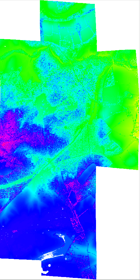
Figure: Mosaic of point cloud data gridded at 2m resolution. Holes (no data) are shown as white

Assuming that there are only small holes in the data set and the DEM is required only within the lidar swath coverage, we can use the r.surf.idw command to interpolate over the lidar. This command will also interpolate into the GRASS region where the LIDAR is undefined.

6. r.surf.idw input=lidar_mosaic output=lidar_mosaic_idw

where the output raster, lidar_mosaic_idw, has been interpolated using an inverse distance weighted formula. As well as filling in holes within the lidar swath, this will also interpolate over empty parts of the GRASS region, resulting in possibly unrealistic data values.

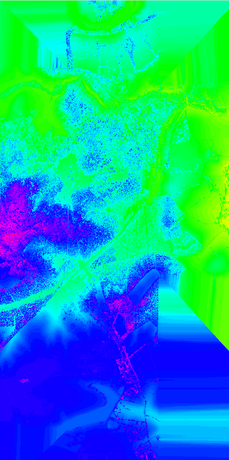
Figure: Interpolated point cloud data over full GRASS region.

This can be improved if you wish by using a mask when interpolating the data. To create a mask, the easiest way is to use your input data at a low resolution. This creates a raster which covers the LIDAR swath but contains no holes in the data (assuming the resolution is selected low enough). To import the data at a lower resolution , repeat steps 1-3 for each ASCII point cloud setting the res variable to a suitable value, e.g. 50.0 and outputting to a new map. Then repeat steps 4 and 5 to create a raster covering the combined LIDAR swath.

Then to use the mask:

7. r.mask input=<maskmapname>

and perform the interpolation step:

8. r.surf.idw input=lidar_mosaic output=lidar_mosaic_idw

this results in a map where the internal holes have been filled, but the area outside the swath coverage remains unchanged.

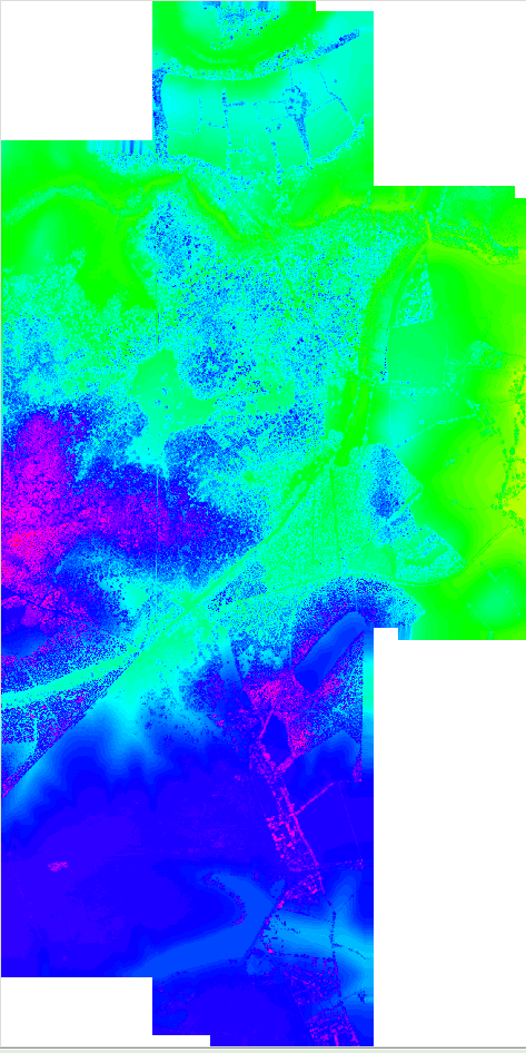
Figure: Interpolated point cloud data after implementing a mask.

To extend the coverage of your DEM, if required, it is suggested to patch on external DEM data. If you have access to a good quality DEM then use that, else the SRTM 3 arc second DEM is freely available and covers most of the globe between +-60 degrees latitude. To see how to make a DEM from SRTM data see the SRTM DEM page. Make sure to select the projection the same as your LIDAR DEM.

Once you have an SRTM DEM of sufficient coverage you can patch the LIDAR and SRTM DEMs together, such that the LIDAR takes precedence. This means the lidar_dem should be the first of the input maps on the r.patch command. If the mask is still applied then remove it before patching:

9. r.mask input=<maskmapname> -r

10. r.patch in=lidar_dem,srtm_dem out=combined_dem

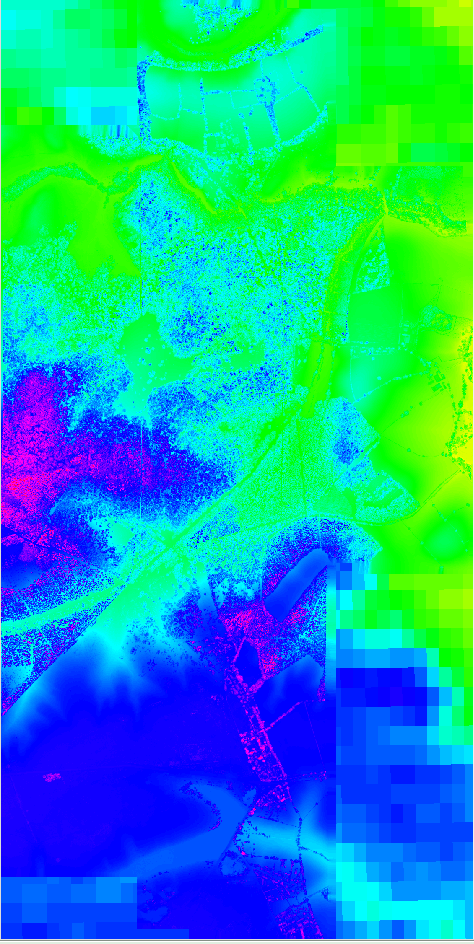
Figure: Interpolated point cloud data after implementing a mask with SRTM DEM data to fill in the rest of the region.

---

Making the DEM suitable for azgcorr

To make a suitable ASCII DEM for use in the azgcorr software, the header information of the ASCII DEM file must be in a certain format. The required format is to have a header of one line (the first line of the file) with the DEM data following. The format is (as given by the azgcorr help):

or c r xm ym xx yx gi

where:

or = row order of the data [0 if South to North, 1 if North to South]

c = number of columns

r = number of rows

xm = minimum easting

ym = minimum northing

xx = maximum easting

yx = maximum northing

gi = grid size (spacing)

An example header, for a DEM of 2000 rows x 2000 columns at 5m resolution, might be: 1 2000 2000 400000 850000 410000 860000 5