| Version 5 (modified by mark1, 14 years ago) (diff) |
|---|
ARSF Hypersectral Data
The ARSF collects hyperspectral data using two instruments, both of which are manufactured by Specim:
- Eagle for visible and near infra-red wavelengths (~400nm to 970nm)
- Hawk for short wave infra-red wavelengths (~1000nm to 2500nm)
The raw data format from these sensors is ENVI band interleaved by line (BIL) files, which is a simple binary data format. Each BIL file comes with an accompanying header file in a human readable text format. The header file contains information about the BIL file format and specifications of the sensor at time of data capture. The Eagle raw data files contain data 12-bit data (0-4095) stored as 16-bit integer, whilst the Hawk raw data are 14-bit (0-16383) stored as 16-bit integer. The first pixel of the first band of each raw file is the frame counter pixel, which is essentially a frame id tag that increments by 1 through out the file. At the end of the raw file, after data capture for this flight line, a number of lines of data are captured with the shutter closed. These lines are refered to as "dark lines" and give sensor ccd values for when no light is present.
When ARSF-DAN receive hyperspectral raw data, it enters the processing chain which consists of the following stages:
- Initial checks and re-formatting project structure
- This includes Digital Elevation Model (DEM) generation
- Aircraft position and navigation post processing
- APL Hyperspectral chain
- Delivery creation
- Delivery checking
- Dispatch Dispatch
After the data has been dispatched to the PI, the project directories will be tidied up and the data archived at the NERC Earth Observation Data Centre (NEODC). The data will then be available for use by other parties after an initial embargo period of 1 year after dispatch.
Hyperspectral processing using the Airborne Processing Library
The Airborne Processing Library (APL) is an open source software package that has been developed by ARSF-DAN at Plymouth Marine Laboratory. It has been specifically designed to process the ARSF Eagle and Hawk data from the raw data collection stage through to end-user geocorrection and mapping. The following gives a description of how ARSF-DAN use APL to process the hyperspectral data upto the point of dispatching the data to the end-user.
Stage 1: Radiometric calibration
The first stage of processing is to apply a radiometric calibration to the raw data and generate a mask file. This can be summarised as follows:
Normalise the data.
The captured dark frames are used to generate a per CCD pixel (i.e. per sample per band) average value which can be used as an effective "0" value. That is, it gives the value of the pixel when no light is shining on the CCD. This is therefore a measure of the noise of the system at time of capture. The raw data is then normalised to this by subtracting the corresponding average dark value. If the value would drop below 0 after subtraction it is set to equal 0.
Smear correct Eagle data
The Eagle uses a CCD that shifts data out line by line at the end of a frame. While this readout process is quick, additional light still falls onto the detector during the readout period. The Eagle data therefore needs to be corrected for any light that is coming from the other bands as the data is extracted. The formula used for this is:
Iic = Ii - f*Sumj<i(Ij)
where Iic is the smear corrected image band i, Ii is the image band i, f is the frame smear correction scalar, Ij is the image band j.
Apply gains
At the start and end of the flying season the Eagle and Hawk instruments are "factory" calibrated. Since 2011 this has been done in-house by ARSF and FSF. One of the products of the instrument calibration is the gain multipliers. This is a per sample list of scalars that convert the sensor captured data value into a "real world" at-sensor radiance value. The image data is multiplied by the corresponding gain value to give the at-sensor radiance value.
Calibrate FODIS if Eagle data
The FODIS collects down-welling light, and is stored on the first 71 pixels of the Eagle CCD. This is calibrated in the same way as the other raw data. When calibrated, the FODIS pixels for the same scan line are averaged together to further reduce random noise.
Insert Missing Scans
Occaisionaly the sensor "drops" a scan line. This can be identified by examining the frame counter through the raw file and observing where it increases by more than 1 between consequetive scans. If a missing scan is identified in the raw image, a dummy scan line of 0s is output to the calibrated image.
Flag Pixels over/under flown, bad, missing
A mask file will be created at the same time that the radiometric calibration is applied. This is a file of the same dimensions as the raw data file that contains the status of each calibrated pixel. The values in the mask file are as follows:
0 - good data
1 - underflown data - the raw value after normalisation is less than 0.
2 - overflown data - the raw value is equal to the maximum (4095 for Eagle, 16383 for Hawk).
4 - bad pixel - usually refers to a Hawk CCD pixel that is considered untrustworthy. Is also used for first 2 pixels of band 1.
8 - Smear affected - a longer wavelength Eagle band has overflown causing the smear correction for this pixel to be incorrect by an unknown quantity.
16 - Dropped scan - a missing scan has been detected and inserted here.
Flipping data and writing
The calibrated data, FODIS and mask files are stored in ENVI BIL format. Prior to writing out, the image data and mask data are reordered. The Eagle data is "flipped" spectrally such that the first band is the lowest wavelength and the last band is the highest (i.e. such that wavelengths are ordered blue to red). The Hawk data is "flipped" spatially such that each scan line is reversed (i.e. pixel 1 becomes pixel 320). This is done because the Eagle and Hawk are mounted backwards to each other and flipping allows targets to be more easily compared between the two sensors data prior to geocorrection.
Stage 2: Navigation - Image syncronising
The second stage of the hyperspectral data processing is concerned with matching up the image scan lines with the sensor orientation and position. The data from the onboard navigation system (currently a Leica IPAS system) are post-processed such that the position and attitude data are blended together to create either a SOL file or SBET file. These files basically contain a list of times together with corresponding GPS location and IMU attitude values.
The Eagle and Hawk sensors also feed off the IPAS navigation system and receive timing pulses. These pulses are used to create a message (sync message) when the sensor starts collecting data, and is stored in the sensor real time navigation file.
APL takes as input these SBET and real time navigation files, together with the calibrated image header information and uses a spline interpolation to get sensor position and attitude for each scan line. It also applies the given sensor boresight and lever arm offset values to the navigation data.
The Eagle and Hawk sensors can suffer from inaccurate timing of the order of ~0.1 seconds. This means that the navigation data and scan lines can be out of sync, which manifests itself as a "wobbly" image. See here for an example. This is currently corrected by eye at ARSF-DAN, processing using time offsets with accuracies of 0.01 seconds.
Stage 3: Geocorrection
This stage of the hyperspectral data processing involves generating a per-pixel list of latitude and longitude values. This is currently only done at ARSF-DAN for quality control and to check the correct navigation syncing has been used. A Digital Elevation Model (DEM) is required to get accurate geocorrection information. The format of the DEM file should be an ENVI file (either BIL or Band sequential (BSQ)) with geographic projection in WGS84 latitude and longitude. The heights should be referenced against the WGS84 spheroid. This is because the GPS navigation is referenced in WGS84 latitude/longitude projection and all other inputs should also be given in this projection to allow direct comparisons.
For each pixel of the scan line, a CCD pixel-to-ground view vector needs to be constructed. This is made up from the sensor view vector and the navigation attitude (which includes the boresight offset). This vector has origin at the sensor, which is given by the synced position since the lever arm offset has been applied. The vector is traversed from the origin until it intersects the DEM surface, at which point the latitude, longitude and height are recorded.
The geocorrection information is written out as a 3-band BIL file (referred to as an IGM file) where the bands are: longitude, latitude and height.
Stage 4: Re-projection
Prior to generating a mapped image it may be best to reproject the data into a more suitable projection, e.g. Transverse Mercator. APL makes use of the open source PROJ libraries for doing reprojection. If the data is collected in the UK and wants to be in Ordnance Survey (OS) National Grid projection, then there is a grid-shift file available to download from the OS website which can be used with PROJ. Typically ARSF-DAN will use either the OS National Grid or Universal Transverse Mercator projection for quality control of the data. The output file has the same format as the previous stage - a 3-band BIL file.
Stage 5: Mapping
The final stage of the hyperspectral data processing is to generate a mapped image. The calibrated image data is taken together with the (reprojected) IGM file so that the image data can be resampled to a regular grid based on the IGM data. The user specifies the pixel size of the output grid and which bands of the image to map.
The mapping is performed in 2 stages. The first of which is to import the IGM file into a tree-like structure to allow more efficient searches based on geographic location. The second stage is to create a regular grid based on the pixel size and IGM projection information, and to iterate across it filling in each cell. The cell is filled with a value based on interpolation of particular image points with regards to distance from the centre of the cell. For example, if nearest neighbour interpolation is used, the nearest image point to the centre of that cell is used to fill the cell.
The map is output as an ENVI BIL file.
Quality control and Delivery creation
When all the flightlines for a project have been processed, the data are quality checked to ensure the correct navigation timing has been used. This consists of processing the data with various navigation timing offsets and examining each one for erroneous wobbles. When the image with the correct timing offset has been identified, this offset is recorded for future reference.
When all timing offsets for all flightlines have been correctly identified the delivery can be created. This is then checked over by another individual to identify any possible errors before dispatch to the end user.
Attachments (3)
-
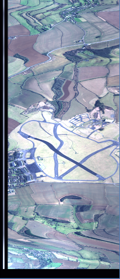
raw_eagle.png
(784.1 KB) -
added by mark1 14 years ago.
Image of raw eagle data including FODIS on left and dark frames at bottom
-
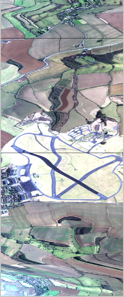
lev1_eagle.png
(812.9 KB) -
added by mark1 14 years ago.
Image of level-1 eagle data
-
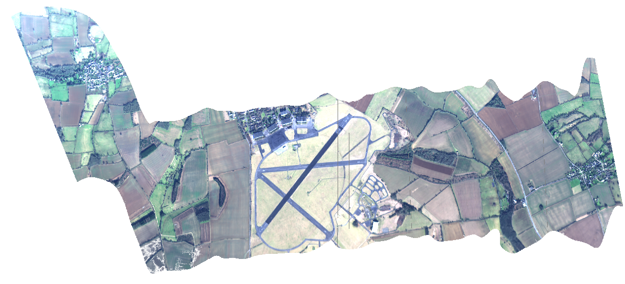
lev3_eagle.png
(745.7 KB) -
added by mark1 14 years ago.
Image of mapped eagle data