Py6S

What is Py6S?

Py6S is an open-source (GPLv3) library that provides an interface to the Second Simulation of the Satellite Signal in the Solar Spectrum (6S) atmospheric Radiative Transfer Model through Python. It was developed by Robin Wilson.

Py6S v1.0 was described in Wilson (2012). You must cite this paper if you use Py6S as part of any research which you later publish: Wilson, R. T., 2012, Py6S: A Python interface to the 6S radiative transfer model, Computers and Geosciences, 51, p166-171. (See what I've done here?)

Documentation is available from: ​https://py6s.readthedocs.org/

There is also a mailing list: ​https://groups.google.com/forum/#!forum/py6s

You can find an overview of ARSF's settings for Py6S model here ARSF's settings for Py6S model here.

Running Py6S for hyperspectral delivery check

You can plot the at-sensor radiance spectra recorded by hyperspectral sensor and compare it to the at-sensor Py6S model using the script check_fenix_spectra_py6s.py. This procedure should be done during the hyperespectral delivery check.

The simplest version of the script looks for a random vegetation pixel at nadir and plots its spectra recorded by the Fenix sensor versus the predefined Py6S vegetation type without atmospheric correction.

Go to delivery project directory that you want to check. Example: ~arsf/arsf_data/2015/flight_data/spain/EUFAR15_38-2015_170_Mallorca/processing/delivery/EUFAR15_38-170-hyperspectral-20151014

If you are airborne user at the selected delivery directory, you can follow the steps on this wiki and simply copy and paste the commands on the terminal.

Create a new folder as airborne user on the temporary directory:

output_folder=/tmp/fenix_vs_py6s-`date +%s`
mkdir $output_folder

You can run several plots per flightline to avoid error caused by a erroneous pixel. You can choose the number of plots to output but suggested number is 3. To run the script select as -i the level1b folder on the delivery created

check_fenix_spectra_py6s.py -i ./flightlines/level1b/  --num_plots 3 -o $output_folder

This will run the Py6S model 3 times for flightline and can take some time to complete. It will create 3 .png files per flightline that you will need to check carefully. To this end, you can find some essential tips on the bottom of this page.

The script also needs the IGM directory and the NAV files for every file on the level1b directory. If the location is not the usual one and the script can't find it, you can specify their paths on the command line by using:

• -m INIGM, --inigm INIGM - Input IGM directory (optional, only required if non-standard location)

• -n INNAV, --innav INNAV - Input post-processed navigation file directory (optional, only required if non-standard location)

If you want to run the model with different settings, click here for more advanced techniques such as:

• Plot spectra for only one flightline in a directory with several ones. Or a specific flightline with different names on IGM, NAV and level1b.
• Chose a pixel by its given (lat, lon).
• Chose a pixel by its position on the grid (x,y).
• Use measured in-situ reflectance instead of the predefined vegetation spectra included in Py6S.

Checking the spectra

The 6S model simulates at-sensor radiance but the parameters used for the atmosphere (atmospheric profile, AOT) are currently kept the same for all times / regions. Therefore, the values of spectra recorded by the Fenix instrument may differ from those produced by Py6S due to differences in actual atmospheric parameters and those used as input to 6S.

Py6S has several parameters needed to run the model. For this script, ARSF have selected the most convenient ones for our use but do not expect perfect match of the hyperspectral spectra recorded from our sensor against the Py6S. A more detailed explanation about Py6S parameters and settings used by ARSF can be found here.

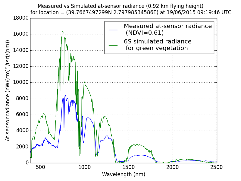
Both curves (Fenix and Py6S) should match general features. The peaks and depression (reflecfance-absorption) caused by vegetation have to match and there should be no other spikes on the Fenix spectra that does not match the Py6s. However, note that it is probably to have a spike on some Fenix spectra flightlines on the bands around band 349, close to 900-950 nm. This is caused by the shift on the SWIR bands detected on on October 2014 and those pixels are listed as bad pixels, therefore the spectra recorded by Fenix is correct. You can find a picture illustrating this issue which also suggest the type of spike you have to look for when they are not on the overlapping region.

Figure above shows Fenix vs Py6S. Both spectra matches except for a Fenix spike close to 980 nm. No other spikes or depressions like that one (which does not match the Py6S model) should be found outside the overlappiing region (around 968-1015 nm). If any other spikes appears outside that region, you will have to check if the spectra is correct using envi and checking those bands have been masked out on the bad pixel list for that flightline.

Moreover, peaks VNIR (around 750-850 nm) and SWIR (1000 nm) has to be present on the Fenix spectra. The SWIR peak should be lower than the VNIR but both of them should be comparable. You can find more detailed examples with pictures about erroneous spectra here.