Airborne Processing Library - Quick Start

This is a short guide aimed at getting users geocorrecting their data straight away. For more in depth information please refer to the APL mapping user guide. The following commands are suitable for use under linux or Microsoft Windows. If running under windows you will need to add '.exe' to the names of the APL programs in the commands below. This assumes that the APL programs are either in the current working directory or in the system path. If you wish to use the GUI then refer to GUI quick start guide

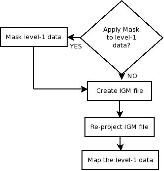
Applying the mask

The delivered level-1 data pixels are not masked if bad - but come with separate mask files. If you wish to apply the mask to the data then you can use the supplied aplmask utility. It is recommended that you apply the mask to your data prior to analysis. An example how to do this:

aplmask -lev1 flightlines/level1b/flightline1.bil -mask flightlines/level1b/flightline1_mask.bil -output flightlines/level1b/flightline1_masked.bil

This will create a masked level-1 file called flightline1_masked.bil where all the 'bad' pixels from the mask file flightline1_mask.bil are set to value '0'. 'Good' pixels will have the value from flightline1.bil.

If you do not wish to mask out every bad pixel but just certain 'varieties', say only overflowed and underflowed pixels, then you can use the '-flags' option. Overflows and underflows have values 1 and 2 in the mask file, and so the following command will only mask these pixels:

aplmask -lev1 flightlines/level1b/flightline1.bil -mask flightlines/level1b/flightline1_mask.bil -output flightlines/level1b/flightline1_masked.bil -flags 1 2

Note that the flags are based on bit values. This means that if a pixel has mask value 10 (smear corrected and overflown) it will be masked out using the above command. To see what pixel values in the mask file represent see here.

Creating an IGM file

An IGM file is a file that contains per-pixel latitude, longitude and height information, and relates directly to the level 1 file. Using the data contained in an ARSF delivery this can be done using the following command for an Eagle image, where the level 1 data file is named flightline1.bil and the output IGM file will be called flightline1.igm. The DEM used is the ASTER DEM as provided with the hyperspectral delivery.

aplcorr -lev1file flightlines/level1b/flightline1.bil -igmfile my_output/flightline1.igm -vvfile sensor_FOV_vectors/eagle_fov_fullccd_vectors.bil -navfile flightlines/navigation/flightline1_nav_post_processed.bil -dem dem/GB11_00-ASTER.dem

We now have per-pixel longitude and latitude values for the level 1 data of file flightline1.bil. But say we want to map the data to a different coordinate system. For this we need to re-project the IGM data.

Reprojection from Geographic Latitude / Longitude

Reprojection is done in APL using the apltran software. This uses the open source PROJ libraries for performing the reprojection. There are 2 projections that have quick keywords set up in apltran; Ordnance Survey National Grid (OSTN02) and WGS84 Universal Transverse Mercator (UTM).

To reproject flightline1.igm into UTM Zone 31 data, using a filename flightline1_utm31.igm we could do the following:

apltran -inproj latlong WGS84 -igm my_output/flightline1.igm -output my_output/flightline1_utm31.igm -outproj utm_wgs84N 31

If we wish to reproject the data into Ordnance Survey National Grid then we must first download the gridshift file from here:

​http://www.ordnancesurvey.co.uk/oswebsite/gps/docs/OSTN02_NTv2_DataFiles.zip

and unzip the files into a directory, say, named ostn02. The file we need has the .gsb extension.

The command to reproject the data into Ordnance Survey National Grid projection is then:

apltran -inproj latlong WGS84 -igm my_output/flightline1.igm -output my_output/flightline1_osng.igm -outproj osng ostn02/OSTN02_NTv2.gsb

It is possible to use any of the PROJ supported projections by using the apltran option -outprojstr followed by the PROJ format projection string. This is out of the scope of this quick start guide but information can be found in the advanced used guide (coming soon).

Gridding the data

We now have per-pixel geolocation information in the required projection. The next and final stage of the mapping procedure is to resample the level 1 data into a regular grid based on the projection information.

The two things we need to decide on are:

• what is a suitable pixel size for the output grid?
• which of the bands do we wish to map?

We can use the ​pixel size estimator to get an idea of the approximate spatial resolution of the data or we can use a different size if we wish. Let us say we want to map using square pixels with 2 metres resolution to match up with some external data we have.

If we wish to map all bands of the level 1 data, and write the data to a file named flightline1_mapped.bil then we can use a command such as:

aplmap -igm my_outputs/flightline1_utm31.igm -lev1 flightlines/level1b/flightline1.bil -mapname my_outputs/flightline1_mapped.bil -pixelsize 2 2 -bandlist ALL

Or if we only want to map a selection of bands, say bands 100 to 150 inclusive, we can use a command such as:

aplmap -igm my_outputs/flightline1_utm31.igm -lev1 flightlines/level1b/flightline1.bil -mapname my_outputs/flightline1_mapped.bil -pixelsize 2 2 -bandlist 100-150