Bullet point notes of Leica training in LIDAR, August 2008.

Leica FTP address: @ftp.leica-geosystems.com

Leica support email: sensors-emea@…

LIDAR nuggets of information

• Doesn't work well in wet conditions
• FOV 0-75 degrees. So an operation at 50 degrees leaves 25 degrees for Roll Compensation
• 75 not recommended since no Roll Compensation and worse results at larger angles.
• Selecting a smaller FOV gives a higher resolution since uses a faster scan rate
• e.g. 24Hz @ 75 degree FOV 90Hz at 1 degree FOV
• With a large FOV shadowing may occur in the data.
• Range gate is (min, max) pulse rates {im not sure of this anymore?}.
  • Maybe the min,max range at which the LIDAR will operate. Will cut off outside this range due to eye safety precautions
• Gaps in the data can occur if LIDAR is operated outside the range gate. (since it shuts down?)
• Data Structure – raw scan data files should all be the same size, except for the last file.
• Log files - “flightline log” is the most useful one to look at. “Laser Current” is not the correct field to look at, instead should be “Laser % Current” that we look at [if we need to know the laser current].
• Ticks per revolution & scan angle correct(ion) are constant (for the system) and never changes.
• Torsion Constant – the flex of the mirror, remains fairly constant at -100000.
• LIDAR has 2 modes of data recording operation, fire mode and BIT (built in test) mode. In BIT mode the laser doesn't actually fire, uses synthetic ranges (needed for calibration flights)
• If have a less then expected % of returns on ALSPP processing output then check the images in TerraScan, look at start/stop times of points at end of flight line – do these match the “flight spreadsheet stuff”. Load up the webcam viewer to see what was below at the point of the flightline where problem has occurred (e.g. Maybe a cloud). If there are no webcam images then operator should have opened the cover! If the flight altitude goes outside of range-gate then system may have shut down for safety purposes.
• IBRC (Intensity based range correction) table – dark objects have a higher correction factor than bright objects since brighter objects reflect faster than dark ones.
• Bright targets can cause problems if surrounded by darker ones (a saturation problem) and can cause approx 20cm elevation errors. These are removed by post-processing filters.
• TPR offset is system specific, depends on the chosen pulse rate. (Our system has -0.116)
• Encoder offset is difference between 0 and the nadir point (exact centre of the scan pattern)
• Pitch error slope is constant/system specific – due to mirror not being perpendicular to the motor rotating it.
• Raw SCaN files contain (among other stuff)
  • Delta Counter (DC) measures the decimal part of time
  • R1-R4 are the ranges in metres of the returns. R4 is always the last return. There is no intensity values for R4.
• If there are less than 4 returns then R4 is an INDEPENDENT measurement of the last pulse received
  • This allows the “average last return” option to be used to give a better measurement (in the ALSPP)
• minimal detectable distance between R1-R2, R2-R3, R3-R4 is 2.7m.

Software stuff

• Aeroplan can help flight planning by giving line spacing, accuracy info, optimisation. Can give expected accuracies for the flight.
• Flight Planning software
  • Aeroplan – LIDAR specific (not licenced),
  • FPES – Generic flight plan software (i.e. Not LIDAR specific)
• Processing Folder Structure – PROJECT NAME
  • IPAS
  • Images
  • RawLaser
  • ProcLaser This structure can be found in the software/workstation/ area of the DVD.
• To do a quick process in ALSPP can use real time navigation. (not recommended for proper processing)
• IPAS Pro.
  • IMU/GPS lever arms output in the extract section should be checked to see if correct (they're entered by operator)
  • The IMU lever arm offset is distance + rotation between IMU and laser
  • The GPS lever arm offset is from Laser to front left corner of LIDAR + distance from GPS antenna to corner (These values can be found on the documents DVD)
  • Check there are no gaps for IMU/GPS data, if there are gaps then they can be located from the GPS times.
• GrafNav.
  • Can open a project and then use autostart
  • Expect +/- 5cm combined separation for short GPS baselines
  • +/-10cm for longer baselines
  • We can copy flight line times into a text file then load camera time marks. This will show flight line time marks on trajectory and graphs
  • Can look at:
    • estimated position accuracy – gives an idea of expected accuracy
    • float/fixed ambiguity – we want fixed
    • Distance separation to see baseline length. For baselines <10km uncheck “use L2 carrier for dual frequency”.
    • RMS of carrier shows how/where the data is bad
    • Look at height profile to get start/stop times when plane is flying level. We should try and select start/stop GPS times when the plane is flying level.
    • Initialise GPS with 3mile straight flight and IMU with a figure of 8 flight – both at start and end of flight. Don't know how useful this actually is. Maybe KAR should be re-initialised just after the figure of 8 loops.
    • GPS for GrafNav- 2Hz MUCH better than 1Hz
    • base station <25km from project location for high quality results
    • PDOP < 2 is best
• ALSPP
  • Average last return should always be used (except when calibrating)
• TerraScan
  • It is possible to synchronise more than one viewer in TerraScan (as in Envi/ERDAS) so can look at intensity and elevation at the same point.
  • We can use TerraScan for creating projects, showing trajectories, splitting and combining LAS files.
  • Create new project – “first button” -> “offset stacked rectangle button”
  • file -> new
    • select LAS storage
    • scanner airborne
    • give description.
  • Place block – allows to draw rectangles to split the data up into sections.
    • Block -> add by boundary
      • will allow to create new LAS files from existing ones.
    • File -> import points into project
      • This does the “splitting” of the data.
  • Can then do things as normal to these project points.
  • Can also recombine all the points to a single LAS file if required.
  • May want trajectory loaded up in TerraScan
    • Setup ALSPP as if to process data.
    • ALSPP -> utilities -> generate trj files.
    • Import into TerraScan and draw trajectory [use the “3 child squares” -> “parallel lines button”to import]
    • The trajectory is important for removing overlaps of data or trimming data and other things.
    • When cutting overlapping points we can use the “by quality” option – low flights take precedence but can also add a quality factor to points which will be used to weight. Alternatively can use the “by offset” option – defines an angle of flightline to cut by.

Calibration procedure

The software DVD contains a project directory structure to use in the calibration procedure.

We should be supplied with factory calibrations of IBRC table, TPR, Encoder stuff.

Boresight/Range correction calibration should take place (approx) 2 times a year.

Calibration flight consists of:

• 2 crosses at different heights (700m and 1350m)
• a line, opposing line and a parallel line (at 2300m)

Need to determine range correction before torsion value. Both give a “smile” effect to the data. (Torsion should be -100000)

• Boresight information.
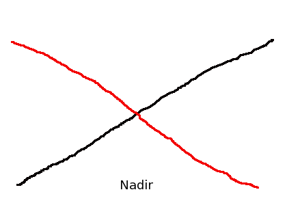
  • Roll – look at 2 opposing strips, swath edges will show height errors (See Figure 1). A runway across swath width is a good target to use for roll detection.
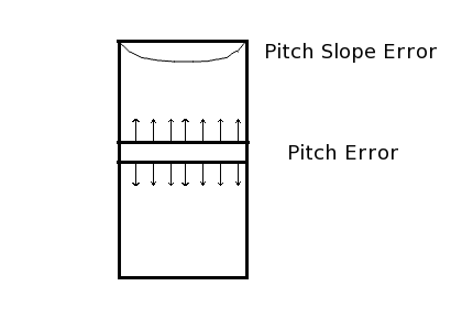
  • Pitch – unnoticeable on flat terrain – need a tilted surface (in the flight direction) and 2 opposing strips. Roof tops can be good targets (See Figure 2)
    • The pitch slope error varies with swath position, 0 at nadir, maximum at edges. Need to check at the centre and the edges of the swath. [This is a different error to the pitch boresight angle]
  • Heading – use parallel lines and a tilting surface (preferably terrain) and paved surfaces (roads/runways).
• The 3 angle corrections can be found using the Attune software
• The pitch slope is found manually during fine tuning/validation of the calibration

The calibration site should have some areas of forest in since want many R2, R3 returns. Need approx 50 tie points in flight line overlap area and another 50 outside. For MPIA flights (that's us) use:

• 750m, 1350m, 2300m altitudes
• Max pulse rate for altitude
• 45 degree FOV
• 120knts air speed
• max scan rate

There should also be around 30-40 visible known ground control points to use for calculating the range offsets in the LIDAR.

Calibration procedure is boresight first, then range correction and finally checks, validation and fine tuning.

PROCEDURE:

• In ALSPP uncheck the “average last returns” option in the settings dialog.
• Check the output as attune files in the outputs dialog
• Add all the flight data into the ALSPP, including the BIT mode data, and run the RangeCardCal program from the utilities menu. Select the use all SCN files option when prompted.
  • This gets the differences for range card banks A & B. Takes differences R1-RL and averages them. Similarly for R2-RL, R3-RL, R4-RL.
• Enter range offset A1 as 0 since it is unknown.
• Enter the output Range offsets into the range corrections dialog of ALSPP. Only need R1 for A and B for now.
• Uncheck the BIT mode data (we don't need to process this) and run the ALSPP processing.
• Look at the filesizes of the output data. If the LAS files are over 400MB in size then Attune will not run. If this is the case re-process with only the part of interest of the line.
  • Part of interest will be the area where all flight lines overlap.
• GROUND CLASSIFICATION NEEDS TO BE DONE HERE
  • See the notes on ground classification
  • we do this so that we only use points on the ground in the tie pointing (since we don't want errors due to perspective or shadowing)
• Start up Attune
• Add ALS data -> add the real ATN.LAS files from the ALSPP output
  • The suggested pixel sizes (from top level calibration pdf) are 0.3m for 750m, 0.4m for 1350m and 0.8m for 2300m.
• View the image pngs to make sure no data holes. (Some are OK. Re-load using a different resolution if too many holes. e.g. Try 0.35m for 750m)
  • 'a' centres the image
  • '+/-' to zoom in/zoom out
• Now select tie points. We use streets for tie points since these should be on the ground so no (little) effects due to look angles and also has slow varying topography
• Open tie point editor in Attune.
  • Press 'm' to measure a point and then click where you want it. Do this for each image (selecting the same point). Then press 'sample all' to record the locations.
  • To change one, re-measure it and then just click 'sample point'.
• Save the project after selecting 50-100 points. (Attune is very crash-able, save often)
• Select points on roads with uniform intensity. Use lines of roads and field boundaries to get the same place in each image. Don't use buildings as markers due to perspective/shadow.
• Edit project file properties.
  • Torsion constant =-100,000
  • Image observation Weights 0.2, 0.2, 0.1
  • Atmosphere same parameters as in the ALSPP processing
  • Set class as ground -> 2 (ground is usually class 2)
  • Adjustment criteria maxiter=50, angular (?)=1.00e-08
• Click Solve Calibration parameters and unselect Torsion, just want to solve roll, pitch and heading.
• Then analyse the adjustment
  • A good result would have aposteriori reference of between 1 and 2.
  • No. of observations of 300 is good
  • Standard deviations of around 0.00001 for Roll and Pitch, 0.00005 for Heading.
  • Average residuals of 25cm for X and Y, 5cm for Z is good.
• If the above criteria are not met (roughly...they are only guidelines)
  • Analyse results and remove or adjust any points with large residuals
    • Open all the images + point editor and then can select a point from the solution list and zoom to it on the images
    • You could just remove the point from one or two images (especially the high altitude images) or from all images. Then recalculate the network adjustment and iterate until Aposteriori reference is approx 1-2 and average residuals are 0.25,0.25 and 0.05.
    • Can remove the points from the lower resolution images if it will help. We want more measurements in the higher resolution images than the lower ones if they are unclear to measure in (so don't just measure in them for the sake of it)
  • When happy save the solution
• Return to ALSPP and add the Roll, Pitch and Heading values to the boresight calibration dialog. Change the outputs to LAS not Attune. Change the output directory too. Re-run the processing.
• Analyse the results in TerraScan
  • Check cross sections etc for misaligning flightlines.
  • To load all flightlines will probably need to use a fence (this is like a region of interest)
  • To check the Roll accuracy – check opposing flights and look at cross sections at either end of the swath for a tilt (across track).
  • To check the Pitch accuracy – check along track on slopes for offsets
  • To check the Heading accuracy – check the parallel lines for offsets
• The boresight parameters can be manually twiddled (rather than using Attune) by reprocessing in ALS, changing the R,P,H values one at time. Only process parts of the flightlines for speed benefits.
• Can now do range correction if the boresight is good. This is a 2 stage process:
  • 1. Nominal offset determination A1
  • 2. Define relative differences for A2,A3,A4 and B1,B2,B3,B4
• points have approx. the same range error within +/-7 degrees of Nadir, so we look only at this region firstly.
  • In ALSPP filters dialog set the angles to +7 and -7 degrees, change the output directory (to 02a_Roff+-7deg if using suggested directory structure) and run the processing on the 4 low altitude flight lines.
  • Load the results into TerraScan and use the 30-40 GCPs of the calibration site.
  • Tools -> Output Control Report
  • Browse -> GCP file and remove bad points (maybe an error occurred in the surveying of a certain point)
  • Look at the dz value, the average dz is used for the nominal range offset A1.
  • Save the text file.
• Preferably using data including areas of forest and the BIT mode data, run RangeCardCal and enter the average dz value as A1 to get the other offsets. Add the outputs to the ALSPP dialog and save the settings reg file (to a new name)
• To check these results re-run using the full FOV (~45 degrees) and check average dz is less than 1cm or so, and standard deviation <5cm in TerraScan control report. (also look at cross sections)
• Then process the 4 high altitude flights in ALSPP and check in TerraScan (around nadir and swath edges)
• Finally load in all flights into TerraScan (within a fence if memory issues) and check them (ideally along a stream because this has a “good” profile) Can use the travel path tool in TerraScan for comparing cross sections along a path.
• Final validation and fine tuning
  • check the torsion and pitch error slope
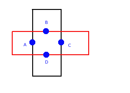
  • To check the Torsion look at cross sections of high altitude cross flight. Flat roads and grassy areas are good. Look for “smiles” in the data. This can be done by looking at the centres of the edges of the overlapping area (Figure 3).
  • We could create a surface model using one of the opposing flight lines, and then difference the other flight line against this to show if there are any roll effects [or maybe torsion etc]. Do this as well as the cross sections.
• When finished save all the results to a reg file in ALSPP

Data QC-ing and processing procedure

We need the air pressure and temperature recorded at a low (ground) and high (aeroplane) altitude over the site. This is to perform the basic atmospheric correction in the ALSPP.

We should start off by calibrating before each flight to check consistency etc. (Just a suggestion though unlikely?) The general processing data QC-ing should primarily take the form of viewing the intensity images to check for striping and to see if they look “correct” i.e. Does it look like the area surveyed. The data should be loaded into TerraScan and checked that all the flight lines line up OK both spatially and vertically (check cross sections around the image).

We may want to do some initial classification (or filtering) of points to remove noisy points, but we shouldn't do a full classification.

For areas that we don't have a good DEM (i.e. Non UK) we may want to generate one to aid the visual instrument processing. Can use TerraScan to create a surface.

Ground Classification

• This is an iterative procedure to take points from default classification to ground classification.
• Classify from default classification to ground.
• Max terrain slope – if lots of man made structures then use 88-90 degrees, else estimate from the natural terrain and add 10-15 degrees.
• To classify, both the vertical distance and angle between points are tested against.
• Its better to classify too few points to ground than too many.
• Its good to preclassify more difficult areas first. [i.e. classify large buildings and steep hill tops].
• In TerraScan load in a LAS file.
• Classify->Routine->ground
  • use measurement tool to get max building size in area. Also for terrain slope can view elevation and use cross section tool to measure/estimate it.
  • Initial points = aerial low and ground
  • iteration angle = 6 degree to start with
  • iteration distance = 1m to start with
• Before ground classification we should remove noisy points.
  • Default -> low points classification.
  • Do this for group of points and then single points.
  • We can set up a macro to do this.
• Set up the Macro
  • Tools -> Macro
  • any -> default
  • default -> low (group)
  • default -> low (single)
  • isolated points -> any -> low
  • To run on large projects use “selected files” instead of reading all into memory.
• Run the macro and check result. Update distances etc used in the classifications if needed.
• Then add ground classification.
  • Default -> ground.
• The Add point to ground tool can be used to add points to the classification that have been missed.
• Can get Model Key Points
  • Routine -> Model key points
  • from ground -> model key points
  • These are the points which can be used as a model (?)

Summary of work required

General information

• Need lever arms from sensor to GPS
  • may be interesting to have lever arm from Applanix to laser too (?)
• Need air pressure and temperature at low and high altitudes

Calibration

• 8 short flight lines in specific pattern over designated site (<400MB each)
• 30-40 known and visible GCP
• boresighting
  • Trajectory processing – 1hr
  • ALS processing multiple times – 1hr
  • Ground classification – 1hr
  • Attune initial tie pointing – 3hr
  • Attune fine tuning – 1hr
• Range corrections – 1-2hr
• Validation and fine tuning – 1hr

General flights

• longer flight lines
  • more processing time
  • harder to QC due to larger file sizes
• ALS processing
• Some classification/noise reduction
• QC checks to see if flight lines line up ok
  • large files may make it difficult and will need to load lines up in sections
• unknown processing times for large flight lines
  • ALS estimate 2-3hrs
  • QCing 2-3hrs

Figure captions

Figure 1. Cross section of opposing flight lines (red and black) with a roll (boresight) error. Small difference between flight lines at nadir, larger error at swath edges.

Figure 2. Plan view of opposing flight lines. A pitch error will result in a (sloped) feature being moved along track, this is easy to spot when comparing cross sections of the opposing flight lines. The pitch slope error causes a “smile effect” to the data.

Figure 3. Check for torsion corrections on a cross flight. Line 1 (black) will see no effect at points B and D, whereas line 2 (red) will show full effect at these points. The opposite is true for points A and C. Using TerraScan to view cross sections at these 4 points should highlight if there is a torsion correction to be made.